Python Package deadwood Reference¶

`deadwood.MSTBase`(*[, M, metric, ...])	A base class for `genieclust.Genie`, `lumbermark.Lumbermark`, `deadwood.Deadwood`, and other Euclidean and mutual reachability minimum spanning tree-based clustering and outlier detection algorithms.
`deadwood.MSTClusterer`([n_clusters, M, ...])	A base class for `genieclust.Genie`, `lumbermark.Lumbermark`, and other spanning tree-based clustering algorithms [1].
`deadwood.MSTOutlierDetector`(*[, M, metric, ...])	A base class for `deadwood.Deadwood` and other spanning tree-based outlier detection algorithms.
`deadwood.Deadwood`(*[, contamination, ...])	Deadwood [1] is an anomaly detection algorithm based on Mutual Reachability Minimum Spanning Trees.
`deadwood.kneedle_increasing`(x[, convex, dt])	Finds the most significant knee/elbow using the Kneedle algorithm [1] with exponential smoothing.
`deadwood.plot_scatter`(X[, y, labels, axis, ...])	Draws a scatter plot.
`deadwood.plot_segments`(pairs, X[, y, style])	Draws a set of disjoint line segments.

deadwood Python Package

class deadwood.Deadwood(*, contamination='auto', max_debris_size='auto', M=5, max_contamination=0.5, ema_dt=0.01, metric='l2', quitefastmst_params=None, verbose=False)¶

Deadwood [1] is an anomaly detection algorithm based on Mutual Reachability Minimum Spanning Trees. It trims protruding tree segments and marks small debris as outliers.

More precisely, the use of a mutual reachability distance [3] pulls peripheral points farther away from each other. Tree edges with weights beyond the detected elbow point [2] are removed. All the resulting connected components whose sizes are smaller than a given threshold are deemed anomalous.

Once the spanning tree is determined (\(\Omega(n \log n)\) – \(O(n^2)\)), the Deadwood algorithm runs in \(O(n)\) time. Memory use is also \(O(n)\).

Parameters:

M, metric, quitefastmst_params, verbose: see deadwood.MSTBase
contamination‘auto’ or float, default=’auto’: The estimated (approximate) proportion of outliers in the dataset. If "auto", the contamination amount will be determined by identifying the most significant elbow point of the curve comprised of increasingly ordered tree edge weights smoothened with an exponential moving average
max_debris_size‘auto’ or int, default=’auto’: The maximal size of leftover connected components that will be considered outliers. If "auto", sqrt(n_samples) is assumed.
max_contaminationfloat, default=0.5: maximal contamination level assumed when contamination is ‘auto’
ema_dtfloat, default=0.01: controls the smoothing parameter \(\alpha = 1-\exp(-dt)\) of the exponential moving average (in edge length elbow point detection), \(y_i = \alpha w_i + (1-\alpha) w_{i-1}\), \(y_1 = d_1\)

Attributes:

n_samples_, n_features_: see deadwood.MSTBase
labels_ndarray of shape (n_samples_,): labels_[i] gives the inlier (1) or outlier (-1) status of the i-th input point.
contamination_float or ndarray of shape (n_clusters_,): Detected contamination threshold(s) (elbow point(s)). For the actual number of outliers detected, compute numpy.mean(labels_<0).
max_debris_size_float: Computed max debris size.
_cut_edges_None or ndarray of shape (n_clusters_-1,): Indexes of MST edges whose removal forms n_clusters_ connected components (clusters) in which outliers are to be sought. This parameter is usually set by fit called on a MSTClusterer.

References

[1] (1,2)

M. Gagolewski, deadwood, in preparation, 2026, TODO

[2]

V. Satopaa, J. Albrecht, D. Irwin, B. Raghavan, Finding a “Kneedle” in a haystack: Detecting knee points in system behavior, In: 31st Intl. Conf. Distributed Computing Systems Workshops, 2011, 166-171, https://doi.org/10.1109/ICDCSW.2011.20

[3]

R.J.G.B. Campello, D. Moulavi, J. Sander, Density-based clustering based on hierarchical density estimates, Lecture Notes in Computer Science 7819, 2013, 160-172, https://doi.org/10.1007/978-3-642-37456-2_14

fit(X, y=None)¶

Detects outliers in a dataset.

Parameters:

Xobject

Typically a matrix or a data frame with n_samples rows and n_features columns; see deadwood.MSTBase.fit_predict for more details.

If X is an instance of deadwood.MSTClusterer (with fit method already invoked), e.g., genieclust.Genie or lumbermark.Lumbermark, then the outliers are sought separately in each detected cluster. Note that this overrides the M, metric, and quitefastmst_params parameters (amongst others).

If X is None, then the outlier detector is applied on the same MST as that determined by the previous call to fit. This way we may try out different values of contamination and max_debris_size much more cheaply.

yNone

Ignored.

Returns:

selfdeadwood.Deadwood: The object that the method was called on.

Notes

Refer to the labels_ attribute for the result.

As with all distance-based methods (this includes local outlier factor as well), applying data preprocessing and feature engineering techniques (e.g., feature scaling, feature selection, dimensionality reduction) might lead to more meaningful results.

class deadwood.MSTBase(*, M=0, metric='l2', quitefastmst_params=None, verbose=False)¶

A base class for genieclust.Genie, lumbermark.Lumbermark, deadwood.Deadwood, and other Euclidean and mutual reachability minimum spanning tree-based clustering and outlier detection algorithms.

A Euclidean minimum spanning tree (MST) provides a computationally convenient representation of a dataset: the n points are connected via n-1 shortest segments. Provided that the dataset has been appropriately preprocessed so that the distances between the points are informative, an MST can be applied in outlier detection, clustering, density estimation, dimensionality reduction, and many other topological data analysis tasks.

Parameters:

Mint, default=0

Smoothing factor for the mutual reachability distance [1]. M = 0 and M = 1 select the original distance as given by the metric parameter.

metricstr, default=’l2’

The metric used to compute the linkage.

One of: "l2" (synonym: "euclidean"; the default), "l1" (synonym: "manhattan", "cityblock"), "cosinesimil" (synonym: "cosine"), or "precomputed".

For "precomputed", the X argument to the fit method must be a distance vector or a square-form distance matrix; see scipy.spatial.distance.pdist.

Determining minimum spanning trees with respect to the Euclidean distance is much faster than with other metrics thanks to the quitefastmst package.

quitefastmst_paramsdict or None, default=None

Additional parameters to be passed to quitefastmst.mst_euclid if metric is "l2".

verbosebool, default=False

Whether to print diagnostic messages and progress information onto stderr.

Attributes:

n_samples_int

The number of points in the dataset.

n_features_int or None

The number of features in the dataset.

labels_ndarray of shape(n_samples_, )

Detected cluster labels or outlier flags.

For clustering, labels_[i] gives the cluster ID of the i-th object (between 0 and n_clusters_ - 1).

For outlier detection, 1 denotes an inlier.

Outliers are labelled -1.

Notes

If metric is "l2", then the MST is computed via a call to quitefastmst.mst_euclid. It is efficient in low-dimensional spaces. Otherwise, a general-purpose implementation of the Jarník (Prim/Dijkstra)-like \(O(n^2)\)-time algorithm is called.

If M > 0, then the minimum spanning tree is computed with respect to a mutual reachability distance [1]: \(d_M(i,j)=\max\{d(i,j), c_M(i), c_M(j)\}\), where \(d(i,j)\) is an ordinary distance and \(c_M(i)\) is the core distance given by \(d(i,k)\) with \(k\) being \(i\)’s \(M\)-th nearest neighbour (not including self, unlike in [1]). This pulls outliers away from their neighbours.

If the distances are not unique, there might be multiple trees spanning a given graph that meet the minimality property.

Environment variables:

OMP_NUM_THREADS: Controls the number of threads used for computing the minimum spanning tree.

References

[1] (1,2,3)

[2]

M. Gagolewski, A. Cena, M. Bartoszuk, Ł. Brzozowski, Clustering with minimum spanning trees: How good can it be?, Journal of Classification 42, 2025, 90-112, https://doi.org/10.1007/s00357-024-09483-1

[3]

M. Gagolewski, quitefastmst, in preparation, 2026, TODO

fit_predict(X, y=None, **kwargs)¶

Performs cluster or anomaly analysis of a dataset and returns the predicted labels.

Refer to fit for a more detailed description.

Parameters:

Xobject: Typically a matrix or a data frame with n_samples rows and n_features columns; see below for more details and options.
yNone: Ignored.
**kwargsdict: Arguments to be passed to fit.

Returns:

labels_ndarray of shape (n_samples_): self.labels_ attribute.

Notes

Acceptable X types are as follows.

If X is None, then the MST is not recomputed; the last spanning tree as well as the corresponding M, metric, and quitefastmst_params parameters are selected.

If X is an instance of MSTBase (or its descendant), all its attributes are copied into the current object (including its MST).

For metric is ‘precomputed’, X should either be a distance vector of length n_samples*(n_samples-1)/2 (see scipy.spatial.distance.pdist) or a square distance matrix of shape (n_samples, n_samples) (see scipy.spatial.distance.squareform).

Otherwise, X should be real-valued matrix (dense numpy.ndarray or an object coercible to) with n_samples rows and n_features columns.

class deadwood.MSTClusterer(n_clusters=2, *, M=0, metric='l2', quitefastmst_params=None, verbose=False)¶

A base class for genieclust.Genie, lumbermark.Lumbermark, and other spanning tree-based clustering algorithms [1].

By removing k-1 edges from a spanning tree, we form k connected components which can be conceived as clusters.

Parameters:

M, metric, quitefastmst_params, verbose: see deadwood.MSTBase
n_clustersint: The number of clusters to detect.

Attributes:

n_samples_, n_features_

see deadwood.MSTBase

labels_ndarray of shape (n_samples_,)

Detected cluster labels.

labels_[i] gives the cluster ID of the i-th input point (between 0 and n_clusters_-1).

Eventual outliers are labelled -1.

n_clusters_int

The actual number of clusters detected by the algorithm.

If it is different from the requested one, a warning is generated.

_cut_edges_ndarray of shape (n_clusters_-1,)

Indexes of the MST edges whose removal forms the n_clusters_ detected connected components (clusters).

References

[1] (1,2)

class deadwood.MSTOutlierDetector(*, M=0, metric='l2', quitefastmst_params=None, verbose=False)¶

A base class for deadwood.Deadwood and other spanning tree-based outlier detection algorithms.

Parameters:

M, metric, quitefastmst_params, verbose: see deadwood.MSTBase

Attributes:

n_samples_, n_features_: see deadwood.MSTBase
labels_ndarray of shape (n_samples_,): labels_[i] gives the inlier (1) or outlier (-1) status of the i-th input point.

deadwood.kneedle_increasing(x, convex=True, dt=0.01)¶

Finds the most significant knee/elbow using the Kneedle algorithm [1] with exponential smoothing.

Parameters:

xndarray: data vector (increasing)
convexbool: whether the data in x are convex-ish (elbow detection) or not (knee lookup)
dtfloat: controls the smoothing parameter \(\alpha = 1-\exp(-dt)\) of the exponential moving average, \(y_i = \alpha x_i + (1-\alpha) x_{i-1}\), \(y_1 = x_1\).

Returns:

indexinteger: the index of the knee/elbow point; 0 if not found

References

[1] (1,2)

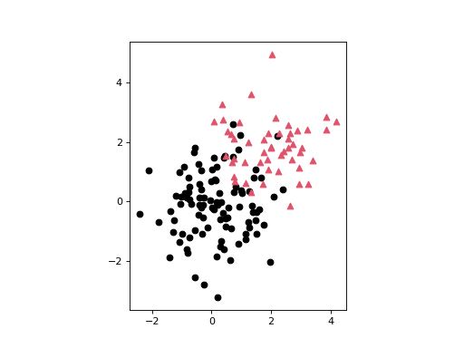
deadwood.plot_scatter(X, y=None, labels=None, axis=None, title=None, xlabel=None, ylabel=None, xlim=None, ylim=None, asp=None, colors=['#000000', '#DF536B', '#61D04F', '#2297E6', '#28E2E5', '#CD0BBC', '#F5C710', '#1f77b4', '#ff7f0e', '#2ca02c', '#d62728', '#9467bd', '#8c564b', '#e377c2', '#7f7f7f', '#bcbd22', '#17becf', '#1f77b4', '#aec7e8', '#ff7f0e', '#ffbb78', '#2ca02c', '#98df8a', '#d62728', '#ff9896', '#9467bd', '#c5b0d5', '#8c564b', '#c49c94', '#e377c2', '#f7b6d2', '#7f7f7f', '#c7c7c7', '#bcbd22', '#dbdb8d', '#17becf', '#9edae5', '#393b79', '#5254a3', '#6b6ecf', '#9c9ede', '#637939', '#8ca252', '#b5cf6b', '#cedb9c', '#8c6d31', '#bd9e39', '#e7ba52', '#e7cb94', '#843c39', '#ad494a', '#d6616b', '#e7969c', '#7b4173', '#a55194', '#ce6dbd', '#de9ed6', '#3182bd', '#6baed6', '#9ecae1', '#c6dbef', '#e6550d', '#fd8d3c', '#fdae6b', '#fdd0a2', '#31a354', '#74c476', '#a1d99b', '#c7e9c0', '#756bb1', '#9e9ac8', '#bcbddc', '#dadaeb', '#636363', '#969696', '#bdbdbd', '#d9d9d9'], markers=['o', '^', '+', 'x', 'D', 'v', 's', '*', '<', '>', '2'], **kwargs)¶

Draws a scatter plot.

Parameters:

Xarray_like: Either a two-column matrix that gives the x and y coordinates of the points or a vector of length n. In the latter case, y must be a vector of length n as well.
yNone or array_like: The y coordinates of the n points in the case where X is a vector.
labelsNone or array_like: A vector of n integer labels that correspond to each point in X, that gives its plot style.
axis, title, xlabel, ylabel, xlim, ylimNone or object: If not None, values passed to matplotlib.pyplot.axis, matplotlib.pyplot.title, etc.
aspNone or object: See matplotlib.axes.Axes.set_aspect.
colorslist: List of colours corresponding to different labels.
markerslist: List of point markers corresponding to different labels.
**kwargsCollection properties: Further arguments to matplotlib.pyplot.scatter.

Notes

If X is a two-column matrix, then plot_scatter(X) is equivalent to plot_scatter(X[:,0], X[:,1]).

Unlike in matplotlib.pyplot.scatter, for any fixed j, all points X[i,:] such that labels[i] == j are always drawn in the same way, no matter the max(labels). In particular, labels 0, 1, 2, and 3 correspond to black, red, green, and blue, respectively.

This function was inspired by the plot() function from the R package graphics.

Examples

An example scatter plots where each point is assigned one of two distinct labels:

>>> n = np.r_[100, 50]
>>> X = np.r_[np.random.randn(n[0], 2), np.random.randn(n[1], 2)+2.0]
>>> l = np.repeat([0, 1], n)
>>> deadwood.plot_scatter(X, labels=l, asp='equal')
>>> plt.show()

(png, hires.png, pdf)

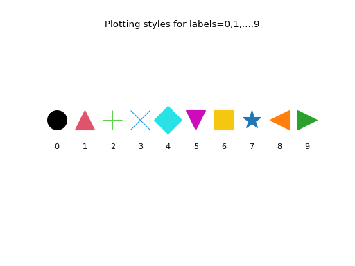
Here are the first 10 plotting styles:

>>> ncol = len(deadwood.colors)
>>> nmrk = len(deadwood.markers)
>>> mrk_recycled = np.tile(
...     deadwood.markers,
...     int(np.ceil(ncol/nmrk)))[:ncol]
>>> for i in range(10):
...     plt.text(
...         i, 0, i, horizontalalignment="center")
...     plt.plot(
...         i, 1, marker=mrk_recycled[i],
...         color=deadwood.colors[i],
...         markersize=25)
>>> plt.title("Plotting styles for labels=0,1,...,9")
>>> plt.ylim(-3,4)
>>> plt.axis("off")
>>> plt.show()

(png, hires.png, pdf)

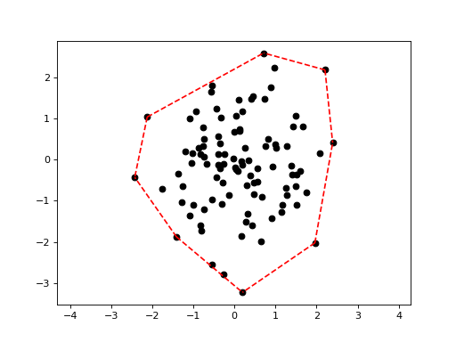
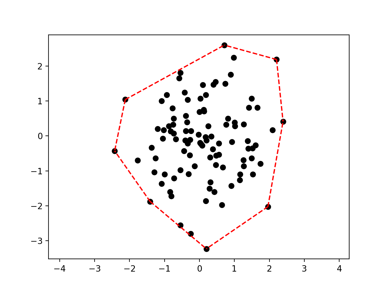
deadwood.plot_segments(pairs, X, y=None, style='k-', **kwargs)¶

Draws a set of disjoint line segments.

Parameters:

pairsarray_like: A two-column matrix that gives the pairs of indexes defining the line segments to draw.
Xarray_like: Either a two-column matrix that gives the x and y coordinates of the points or a vector of length n. In the latter case, y must be a vector of length n as well.
yNone or array_like: The y coordinates of the n points in the case where X is a vector.
style:: See matplotlib.pyplot.plot.
**kwargsCollection properties: Further arguments to matplotlib.pyplot.plot.

Notes

The function draws a set of disjoint line segments from (X[pairs[i,0],0], X[pairs[i,0],1]) to (X[pairs[i,1],0], X[pairs[i,1],1]) for all i from 0 to pairs.shape[0]-1.

matplotlib.pyplot.plot is called only once. Therefore, you can expect it to be pretty fast.

Examples

Plotting the convex hull of a point set:

>>> import scipy.spatial
>>> X = np.random.randn(100, 2)
>>> hull = scipy.spatial.ConvexHull(X)
>>> deadwood.plot_scatter(X)
>>> deadwood.plot_segments(hull.simplices, X, style="r--")
>>> plt.axis("equal")
>>> plt.show()

(png, hires.png, pdf)

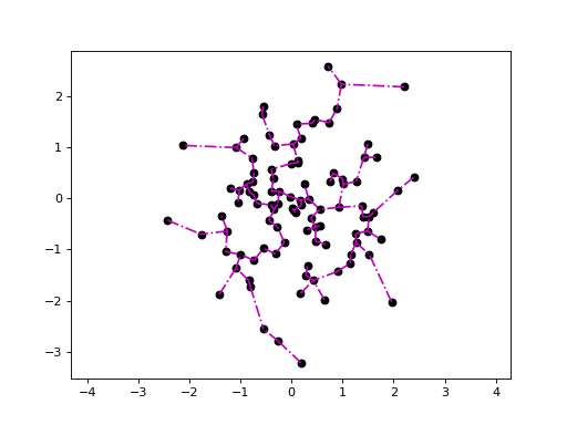
Plotting the Euclidean minimum spanning tree:

>>> import quitefastmst
>>> X = np.random.randn(100, 2)
>>> mst = quitefastmst.mst_euclid(X)
>>> deadwood.plot_scatter(X)
>>> deadwood.plot_segments(mst[1], X, style="m-.")
>>> plt.axis("equal")
>>> plt.show()

(png, hires.png, pdf)