deadwood: Deadwood: Outlier Detection via Trimming of Mutual Reachability Minimum Spanning Trees¶

Description¶

Deadwood is an anomaly detection algorithm based on Mutual Reachability Minimum Spanning Trees. It trims protruding tree segments and marks small debris as outliers.

More precisely, the use of a mutual reachability distance pulls peripheral points farther away from each other. Tree edges with weights beyond the detected elbow point are removed. All the resulting connected components whose sizes are smaller than a given threshold are deemed anomalous.

Usage¶

deadwood(d, ...)

## Default S3 method:
deadwood(
  d,
  M = 5L,
  contamination = NA_real_,
  max_debris_size = NA_real_,
  max_contamination = 0.5,
  ema_dt = 0.01,
  distance = c("euclidean", "l2", "manhattan", "cityblock", "l1", "cosine"),
  verbose = FALSE,
  ...
)

## S3 method for class 'dist'
deadwood(
  d,
  M = 5L,
  contamination = NA_real_,
  max_debris_size = NA_real_,
  max_contamination = 0.5,
  ema_dt = 0.01,
  verbose = FALSE,
  ...
)

## S3 method for class 'mstclust'
deadwood(
  d,
  contamination = NA_real_,
  max_debris_size = NA_real_,
  max_contamination = 0.5,
  ema_dt = 0.01,
  verbose = FALSE,
  ...
)

## S3 method for class 'mst'
deadwood(
  d,
  contamination = NA_real_,
  max_debris_size = NA_real_,
  max_contamination = 0.5,
  ema_dt = 0.01,
  cut_edges = NULL,
  verbose = FALSE,
  ...
)

Arguments¶


`d`	a numeric matrix with \(n\) rows and \(p\) columns (or an object coercible to one, e.g., a data frame with numeric-like columns), an object of class `dist` (see `dist`), an object of class `mstclust` (see genieclust and lumbermark), or an object of class `mst` (see `mst`)
`...`	further arguments passed to `mst`
`M`	smoothing factor; \(M \leq 1\) gives the selected `distance`; otherwise, the mutual reachability distance based on the \(M\)-th nearest neighbours is used
`contamination`	single numeric value or `NA`; the estimated (approximate) proportion of outliers in the dataset; if `NA`, the contamination amount will be determined by identifying the most significant elbow point of the curve comprised of increasingly ordered tree edge weights smoothened with an exponential moving average
`max_debris_size`	single integer value or `NA`; the maximal size of the leftover connected components that will be considered outliers; if `NA`, \(\sqrt{n}\) is assumed
`max_contamination`	single numeric value; maximal contamination level assumed when `contamination` is `NA`
`ema_dt`	single numeric value; controls the smoothing parameter \(\alpha = 1-\exp(-dt)\) of the exponential moving average (in edge length elbow point detection), \(y_i = \alpha w_i + (1-\alpha) w_{i-1}\), \(y_1 = d_1\)
`distance`	metric used in the case where `d` is a matrix; one of: `"euclidean"` (synonym: `"l2"`), `"manhattan"` (a.k.a. `"l1"` and `"cityblock"`), `"cosine"`
`verbose`	logical; whether to print diagnostic messages and progress information
`cut_edges`	numeric vector or `NULL`; \(k-1\) indexes of the tree edges whose omission lead to \(k\) connected components (clusters), where the outliers are to be sought independently; most frequently this is generated via genieclust or lumbermark.

Details¶

As with all distance-based methods (this includes k-means and DBSCAN as well), applying data preprocessing and feature engineering techniques (e.g., feature scaling, feature selection, dimensionality reduction) might lead to more meaningful results.

If d is a numeric matrix or an object of class dist, mst will be called to compute an MST, which generally takes at most \(O(n^2)\) time. However, by default, for low-dimensional Euclidean spaces, a faster algorithm based on K-d trees is selected automatically; see mst_euclid from the quitefastmst package.

Once the spanning tree is determined (\(\Omega(n \log n)\)-\(O(n^2)\)), the Deadwood algorithm runs in \(O(n)\) time. Memory use is also \(O(n)\).

Value¶

A logical vector y of length \(n\), where y[i] == TRUE means that the i-th observation is deemed to be an outlier.

The mst attribute gives the computed minimum spanning tree which can be reused in further calls to the functions from genieclust, lumbermark, and deadwood. cut_edges gives the cut_edges passed as argument. contamination gives the detected contamination levels in each cluster (which can be different from the observed proportion of outliers detected).

Author(s)¶

Marek Gagolewski

References¶

M. Gagolewski, deadwood, in preparation, 2026, TODO

V. Satopaa, J. Albrecht, D. Irwin, B. Raghavan, Finding a “Kneedle” in a haystack: Detecting knee points in system behavior, In: 31st Intl. Conf. Distributed Computing Systems Workshops, 2011, 166-171, doi:10.1109/ICDCSW.2011.20

R.J.G.B. Campello, D. Moulavi, J. Sander, Density-based clustering based on hierarchical density estimates, Lecture Notes in Computer Science 7819, 2013, 160-172, doi:10.1007/978-3-642-37456-2_14

Examples¶

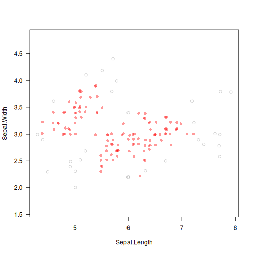
library("datasets")
data("iris")
X <- jitter(as.matrix(iris[1:2]))  # some data
is_outlier <- deadwood(X, M=5)
plot(X, col=c("#ff000066", "#55555555")[is_outlier+1],
    pch=c(16, 1)[is_outlier+1], asp=1, las=1)

plot of chunk deadwood