Comparing Algorithms on Toy Datasets

The scikit-learn homepage showcases a couple of outlier detection algorithms on 2D toy datasets. Below we re-run this illustration on a larger data sample and with the Deadwood algorithm included.

TL;DR — See the bottom of the page for the resulting figure.

import time
import warnings
import numpy as np
import matplotlib.pyplot as plt
import pandas as pd
from sklearn import svm
from sklearn.covariance import EllipticEnvelope
from sklearn.datasets import make_blobs, make_moons
from sklearn.ensemble import IsolationForest
from sklearn.kernel_approximation import Nystroem
from sklearn.linear_model import SGDOneClassSVM
from sklearn.neighbors import LocalOutlierFactor
from sklearn.pipeline import make_pipeline
import deadwood

np.random.seed(1234)

First, we generate the datasets. Note that in the original script, n_samples was set to 300.

n_samples = 3_000
outliers_fraction = 0.15
n_outliers = int(outliers_fraction * n_samples)
n_inliers = n_samples - n_outliers

blobs_params = dict(random_state=0, n_samples=n_inliers, n_features=2)
datasets = [
    make_blobs(centers=[[0, 0], [0, 0]], cluster_std=0.5, **blobs_params)[0],
    make_blobs(centers=[[2, 2], [-2, -2]], cluster_std=[0.5, 0.5], **blobs_params)[0],
    make_blobs(centers=[[2, 2], [-2, -2]], cluster_std=[1.5, 0.3], **blobs_params)[0],
    4.0
    * (
        make_moons(n_samples=n_samples, noise=0.05, random_state=0)[0]
        - np.array([0.5, 0.25])
    ),
    14.0 * (np.random.RandomState(42).rand(n_samples, 2) - 0.5),
]

Here are the method definitions:

anomaly_algorithms = [
    (
        "Deadwood",
        deadwood.Deadwood(contamination=outliers_fraction),
    ),
    (
        "Local Outlier Factor",
        LocalOutlierFactor(n_neighbors=35, contamination=outliers_fraction),
    ),
    (
        "Robust covariance",
        EllipticEnvelope(contamination=outliers_fraction, random_state=42),
    ),
    ("One-Class SVM", svm.OneClassSVM(nu=outliers_fraction, kernel="rbf", gamma=0.1)),
    (
        "One-Class SVM (SGD)",
        make_pipeline(
            Nystroem(gamma=0.1, random_state=42, n_components=150),
            SGDOneClassSVM(
                nu=outliers_fraction,
                shuffle=True,
                fit_intercept=True,
                random_state=42,
                tol=1e-6,
            ),
        ),
    ),
    (
        "Isolation Forest",
        IsolationForest(contamination=outliers_fraction, random_state=42),
    ),
]

Let’s apply the methods on benchmark data:

plt.figure(figsize=(len(anomaly_algorithms) * 2 + 4, 14.5))
plt.subplots_adjust(
    left=0.02, right=0.98, bottom=0.001, top=0.96, wspace=0.05, hspace=0.01
)

plot_num = 1
rng = np.random.RandomState(42)

for i_dataset, X in enumerate(datasets):
    # Add outliers
    X = np.concatenate([X, rng.uniform(low=-6, high=6, size=(n_outliers, 2))], axis=0)

    for name, algorithm in anomaly_algorithms:
        t0 = time.time()
        algorithm.fit(X)
        t1 = time.time()
        plt.subplot(len(datasets), len(anomaly_algorithms), plot_num)
        if i_dataset == 0:
            plt.title(name, size=18)

        # fit the data and tag outliers
        if name in ["Local Outlier Factor", "Deadwood"]:
            y_pred = algorithm.fit_predict(X)
        else:
            y_pred = algorithm.fit(X).predict(X)

        colors = np.array(["#377eb8", "#ff7f00"])
        plt.scatter(X[:, 0], X[:, 1], s=10, color=colors[(y_pred + 1) // 2])

        plt.xlim(-7, 7)
        plt.ylim(-7, 7)
        plt.axis("equal")
        plt.xticks(())
        plt.yticks(())
        plt.text(
            0.99,
            0.01,
            ("%.2fs" % (t1 - t0)).lstrip("0"),
            transform=plt.gca().transAxes,
            size=15,
            horizontalalignment="right",
        )
        plot_num += 1

plt.show()

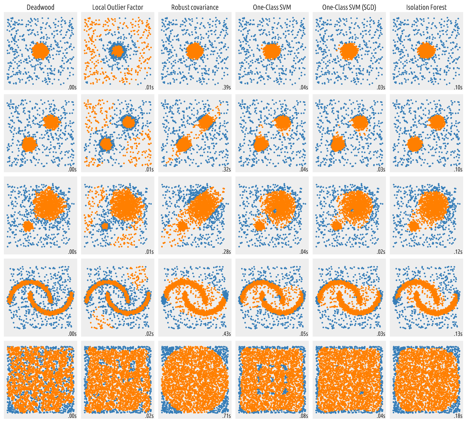
Figure 6 Outputs of outlier detection algorithms

The Deadwood method generates quite meaningful partitions. It is also the fastest among the above ones. Even though no algorithm is perfect in all the possible scenarios, Deadwood is definitely worth a try in your next data mining challenge.

As with all distance-based methods (this includes local outlier factor as well), applying data preprocessing and feature engineering techniques (e.g., feature scaling, feature selection, dimensionality reduction) might lead to more meaningful results.